In this tutorial, we have an Excel file with data about suppliers and we want to find out how many suppliers there are in each city and what number of employees the suppliers have in each city. To achieve this, we will build an automation that creates a pivot table.

Step 1: Set up the project and get the necessary files

1. Create a new project using the default settings.
2. Download and extract the archive with the automation project in this tutorial using the button at the bottom of this page and copy the file Suppliers.xlsx to your project folder.

Step 2: Add the Excel file to the project.

1. Click on the Designer panel.
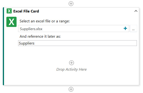
2. In the Common Scenarios section of the search box at the top of the screen, double-click Use Excel File and then browse to and select the file Suppliers.xlsx. An Excel File Card activity is added to the Designer panel.
3. In the activity, in the field And reference it later as enter Suppliers.
   You have indicated that you will work on the file Suppliers.xlsx that is known in your automation as Suppliers.

Step 3: Add and configure the Create Pivot Table activity.

1. In the Excel File Card, click , then find the Create Pivot Table activity in the search box at the top of the screen and double-click it. The activity is added inside the Excel File Card.
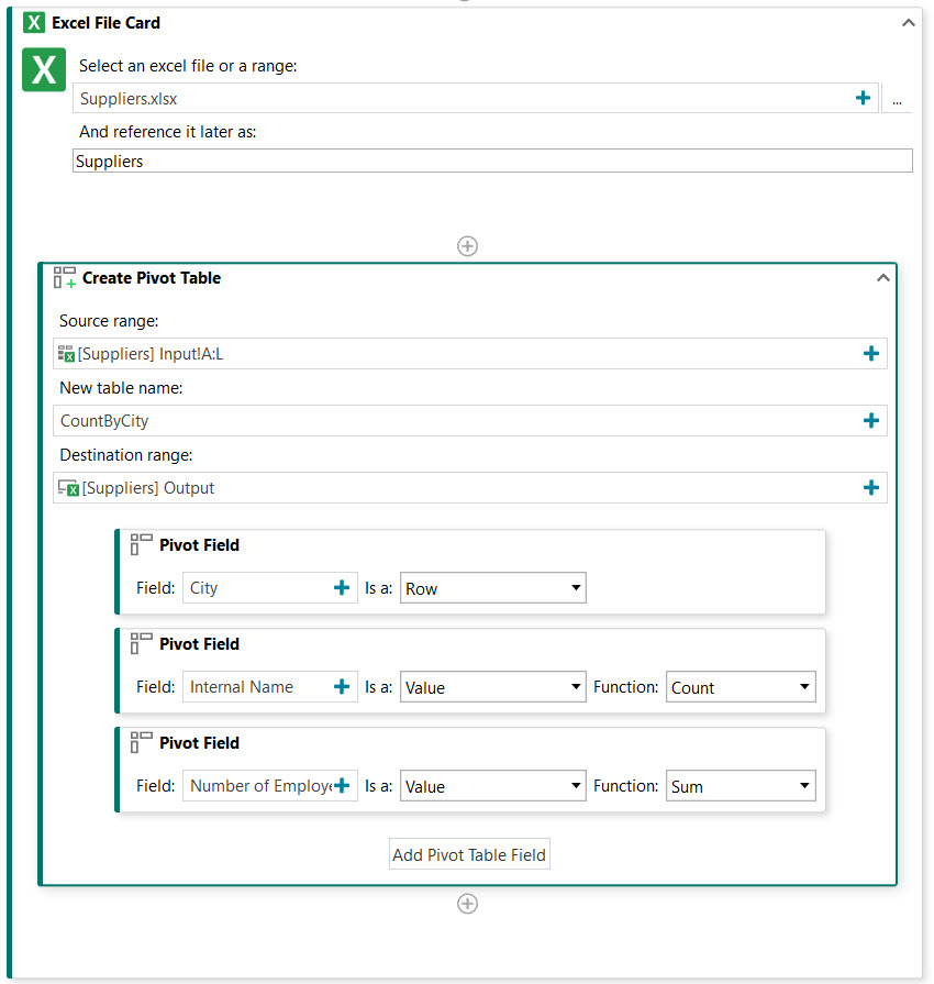
2. In the Create Pivot Table activity, define the source range and the range where to create the pivot table:
   a) Click on the right side of the Source range field and then select Suppliers > Indicate in Excel.
   b) In the Excel file, select all the columns in the Input sheet and then click Confirm in the UiPath tab in the Excel ribbon menu.
   You have indicated that you want to create a pivot table for columns A-L in the sheet named Input in the Excel file referenced as Suppliers. The Table range field displays your selection as [Suppliers] Input!A:L.
   c) Click on the right side of the New table name field and then select Text. In the Text Builder window, enter a name for the pivot table, for example CountByCity and click Save.
   d) Click on the right side of the Destination range field and then select Suppliers > Output [Sheet].
   You have indicated that you want to create the pivot table in the sheet named Output in the Excel file referenced as Suppliers. The Destination range field displays your selection as [Suppliers] Output.
3. In the Create Pivot Table activity, add the pivot table fields:
   a) Click the Add Pivot Table Field button, then click on the right side of Field and select Column Name > City.
   b) From the Is a drop-down menu, select Row.
   You have indicated that you want the entries in the City column in the sheet named Input in the Excel file referenced as Suppliers to be rows in your pivot table.
   c) Click the Add Pivot Table Field button again to add a second field in the pivot table to count the suppliers.
   In the second Pivot Field, click on the right side of Field and then select Column Name > Internal Name.
   d) From the Is a drop-down menu, select Value, and then, from the Function drop-down menu, select Count.
   You have indicated that you want to count the suppliers identified by the column Internal Name in the sheet named Input in the Excel file referenced as Suppliers.
   e) Click the Add Pivot Table Field button again to add a third field in the pivot table to sum up the number of employees.
   In the third Pivot Field, click on the right side of Field and then select Column Name > Number of Employees.
   f) From the Is a drop-down menu, select Value, and then, from the Function drop-down menu, select Sum.
   You have indicated that you want to sum up the number of employees in the sheet named Input in the Excel file referenced as Suppliers.

4. Click Save in the ribbon menu to save the automation, then click Run to execute the automation.

The pivot table is created in the Output sheet of the Suppliers.xlsx file.

Download example